Abstract
This paper presents a performance enhanced Risk-Aware Model Predictive Path Integral (RA‑MPPI) control using Gaussian-process (GP). To this end, the real system is run with arbitrary control input and the resulting data is saved. Based on the nominal model of the system and the collected data, uncertainty affecting the state transition is estimated by a Jacobian-based method offline. Then, the used control input and the estimated uncertainty are used to train the Gaussian process which generates the mean and variance of the uncertainty. Online, the gap between the nominal and real dynamics is compensated by the trained GP. In other words, the nominal model is refined using the estimated noise mean, while the estimated noise variance is directly incorporated into the RA‑MPPI framework, eliminating the need to manually tune the disturbance covariance parameter. Validation is conducted through simulation experiments in Gazebo using a F1TENTH car with a bicycle model navigating a track with and without obstacles. Also, real‑world performance is further demonstrated on the F1TENTH car platform driving the same track under similar conditions. Across both simulation and real‑world scenarios, the proposed method demonstrates improved safety and trajectory tracking performance compared to baseline MPPI and RA‑MPPI techniques in terms of lap times and the number of crash‑free lap completions. Videos of the F1TENTH car simulations, experiments, and similar Gazebo simulation results using a Clearpath Jackal with a differential drive model are available at the project webpage: https://gp-ramppi.github.io.
The proposed method (summarized)
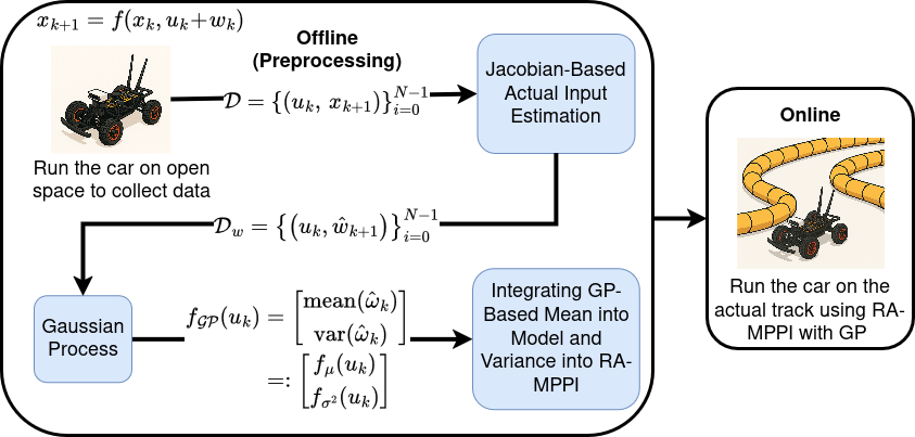
Offline
- Collect data in open space. Drive the robot in open space manually or with a simple controller (e.g., baseline MPPI) at speeds/trajectories similar to the target task and log pairs \( (u_k, x_{k+1}) \) to form the dataset \( \mathcal{D}=\{(u_k,x_{k+1})\}_{k=0}^{N-1} \).
-
Estimate actual input and lumped uncertainty (Jacobian-based).
For each sample \(k\), initialize \(u_{\mathrm{act},k}^{(0)} = u_k\) and iterate:
where \(J=\partial f/\partial u\) and \(^{\dagger}\) denotes the pseudo-inverse. After convergence, compute the lumped input-channel uncertainty \( \hat{w}_k = u_k - \hat{u}_{\mathrm{act},k} \), and build \( \mathcal{D}_w=\{(u_k,\hat{w}_k)\}_{k=0}^{N-1} \).
- \(\hat{x}_{k+1}^{(i)} = f(x_k,\;u_{\mathrm{act},k}^{(i)})\)
- \(\Delta x_k^{(i)} = x_{k+1} - \hat{x}_{k+1}^{(i)}\)
- \(\delta u^{(i)} = J\!\big(x_k,u_{\mathrm{act},k}^{(i)}\big)^{\dagger}\,\Delta x_k^{(i)}\)
- \(u_{\mathrm{act},k}^{(i+1)} = u_{\mathrm{act},k}^{(i)} + \alpha\,\delta u^{(i)},\ (0<\alpha\le 1)\)
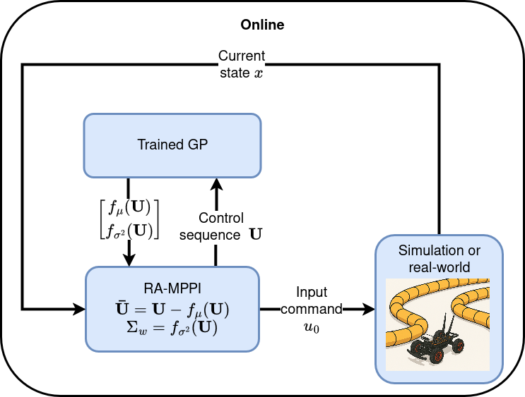
- Train Gaussian Processes per input channel. Fit \(n_u\) independent GPs (RBF kernel) on \( \mathcal{D}_w \) to learn \( u \mapsto w \). Hyperparameters (e.g., \( \sigma_f, \ell \)) are optimized via negative log marginal likelihood minimization. The trained models return, for any input \(u\), a mean \( f_{\mu}(u) \) and variance \( f_{\sigma^2}(u) \) of the uncertainty: \( f_{\mathcal{GP}}(u) \sim \mathcal{N}\!\big(f_{\mu}(u),\,f_{\sigma^2}(u)\big) \).
Online
Application to Mobile Robot
F1TENTH
Model
- The robot is modeled as a bicycle model with state \( x = (p_x, p_y, \theta) \) (position and heading).
- The control inputs are \( u = (v, \delta) \), where \(v\) is the velocity and \(\delta\) is the steering angle.
- With sampling time \(T_s\), the discrete-time kinematics are: $$\begin{aligned} p_{x,k+1} &= p_{x,k} + T_s\, v_k \cos(\theta_k),\\ p_{y,k+1} &= p_{y,k} + T_s\, v_k \sin(\theta_k),\\ \theta_{k+1} &= \theta_k + T_s\,\frac{v_k}{L}\,\tan(\delta_k), \end{aligned}$$ where \(L\) is the wheelbase of the vehicle (constant for the F1TENTH car).
Gazebo Simulation Evaluation
Parameters
- Sampling rate: 50.0 Hz (Ts = 0.02 s)
- Time horizon: 1.5 s (Prediction horizon K = 75 steps)
- Number of trajectories: M = 256
- Exploration variance: γ = 1200.0
- Control covariance: Σv = diag(0.3², 0.4²)
- Inverse temperature: λ = 0.01
- State weights: W = diag(1, 1, 0)
- Control weights: R = λ Σv−1/2
- Collision cost: Ccol = 10⁷
- Max velocity: 3 m/s
- Max steer: 1 rad
- RA-MPPI number of aware trajectories: N = 16
- RA-MPPI weight parameters: A = 0.1, B = 0.9
Real-World Evaluation
Parameters
- All components of the control stack—cost function, Jacobian-based uncertainty estimation, Gaussian process (GP) training, evaluation metrics, and controller parameters—remain similar to those used in simulation.
- Only the controller's sampling rate is adjusted to 20.0 Hz (Ts = 0.05 s), and the control covariance is set to Σv = diag(0.3², 0.3²), to accommodate differences in the hardware platform and slight variations in vehicle dynamics.
Clearpath Jackal
Model
- The robot is modeled as a differential drive with state \( x = (p_x, p_y, \theta) \) (position and heading).
- The control inputs are \( u = (v, \omega) \), where \(v\) is linear velocity and \(\omega\) is angular velocity.
- With sampling time \(T_s\), the discrete-time kinematics are: $$\begin{aligned} p_{x,k+1} &= p_{x,k} + T_s\, v_k \cos\theta_k,\\ p_{y,k+1} &= p_{y,k} + T_s\, v_k \sin\theta_k,\\ \theta_{k+1} &= \theta_k + T_s\, \omega_k. \end{aligned}$$
Gazebo Simulation
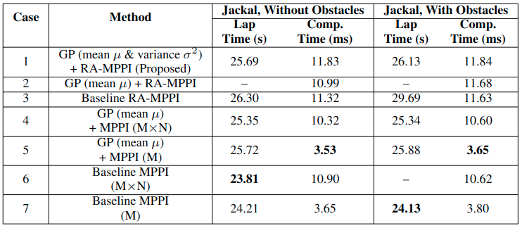
Result
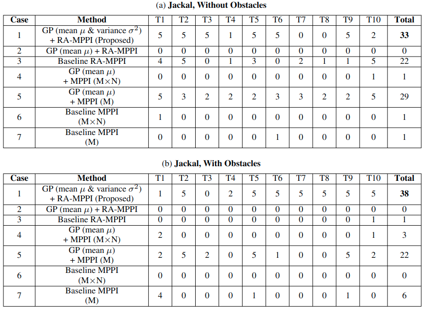
Analysis
- MPPI that use the GP mean tend to increase the number of completed laps (especially Case 5) compared to the baseline MPPI methods (Cases 6 and 7).
- By leveraging both the GP mean and variance (the proposed method, Case 1), the system achieves the highest number of completed laps while maintaining competitive speed.
- The proposed method demonstrates computation times comparable to those of MPPI with \(M \times N\) trajectories and RA-MPPI (Cases 2, 3, 4, and 6).
Appendix: Convergence Analysis of the Gauss-Newton Uncertainty Estimation Iteration
Theorem Statement
Consider the discrete-time system $$ x_{k+1} = f(x_k, u_{\mathrm{act}}), $$ where $x_k \in \mathbb{R}^{n_x}$ is the state at time step $k$, $u_{\mathrm{act}} \in \mathbb{R}^{n_u}$ the actual control input, and $f$ a sufficiently smooth function describing the known nominal model. The goal is to identify $u_{\mathrm{act}}$ by solving $$ x_{k+1} - f(x_k, u) = 0. $$
Define the residual function $$ \mathbf{r}(u) = x_{k+1} - f(x_k, u), $$ so that we seek $u^* = u_{\mathrm{act}}$ satisfying $\mathbf{r}(u^*) = 0$.
The iterative update rule is $$ u^{(i+1)} = u^{(i)} + \alpha J^{\dagger}(u^{(i)})\, \mathbf{r}(u^{(i)}), $$ where $J = \partial f / \partial u$ and $J^{\dagger}$ is the Moore–Penrose pseudoinverse.
Theorem: Under standard smoothness conditions, proper step size $\alpha$, and an initial guess sufficiently close to $u^*$, this iteration converges locally to $u^*$ if $$ \| I_{n_u} - \alpha J^{\dagger}(u^*) J(u^*) \| < 1. $$
Proof
The proof proceeds via a fixed-point contraction argument...
Fixed-Point View
Define $$ \mathbf{G}(u) = u + \alpha J^{\dagger}(u)[x_{k+1} - f(x_k,u)], $$ so a solution satisfies $\mathbf{G}(u^*) = u^*$.
Local Convergence Criterion
The Jacobian of $\mathbf{G}$ near $u^*$ satisfies approximately $$ D\mathbf{G}(u^*) \approx I_{n_u} - \alpha J^{\dagger}(u^*) J(u^*). $$ Local contraction holds if its norm is strictly less than 1.
Computing $D\mathbf{G}(u^*)$
Since $\partial \mathbf{r} / \partial u = -J$, one obtains $$ D\mathbf{G}(u^*) \approx I_{n_u} - \alpha J^{\dagger}(u^*) J(u^*). $$
Local Convergence Under the Condition
If $$ \| I_{n_u} - \alpha J^{\dagger}(u^*) J(u^*) \| < 1, $$ then $\mathbf{G}$ is locally contractive, and the iteration converges to $u^*$.
Why the Condition Often Holds
If $J(u^*)$ has full column rank, then $$ J^{\dagger}(u^*) J(u^*) = I_{n_u}, $$ leading to $$ \| (1-\alpha)I_{n_u} \| = |1-\alpha| < 1 \quad (\alpha>0). $$
Overdetermined or Underdetermined Cases
The iteration still converges if the Jacobian has full column (overdetermined) or row (underdetermined) rank, ensuring proper least-squares or minimum-norm updates.